Anybody interested in building their own robot, sending spacecraft to the moon, or launching inter-continental ballistic missiles should have at least some basic filter options in their toolkit, otherwise the robot will likely wobble about erratically and the missile will miss it’s target.
What is a filter anyway? In practical terms, the filter should smooth out erratic sensor data with as little time lag, or ‘error lag’ as possible. In the case of the missile, it could travel nice and smoothly through the air, but miss it’s target because the positional data is getting processed ‘too late’. The simplest filter, that many of us will have already used, is to pause our code, take about 10 quick readings from our sensor and then calculate the mean by dividing by 10. Incredibly simple and effective as long as our machine or process is not time sensitive – perfect for a weather station temperature sensor, although wind direction is slightly more complicated. A wind vane is actually an example of a good sensor giving ‘noisy’ readings: not that the sensor itself is noisy, but that wind is inherently gusty and is constantly changing direction.

It’s a really good idea to try and model our data on some kind of computer running software that will print out graphs – I chose the Raspberry Pi and installed Jupyter Notebook running Python 3.
The photo on the left shows my test rig. There’s a PT100 probe with it’s MAX31865 break-out board, a Dallas DS18B20 and a DHT22. The shield on the Pi is a GPS shield which is currently not used. If you don’t want the hassle of setting up these probes there’s a Jupyter Notebook file that can also use the internal temp sensor in the Raspberry Pi. It’s incredibly quick and easy to get up and running.
It’s quite interesting to see the performance of the different sensors, but I quickly ended up completely mangling the data from the DS18B20 by artificially adding randomly generated noise and some very nasty data spikes to really punish the filters as much as possible. Getting the temperature data to change rapidly was effected by putting a small piece of frozen Bockwurst on top of the DS18B20 and then removing it again.
Although, for convenience, I derived data from a temperature sensor, a moving machine such as a robot would be getting data from an accelerometer and probably an optical encoder and a filter that updates ‘on the fly’ is essential.
Moving Averages
The simplest form is what’s called the ‘Simple Moving Average’ (SMA), which is similar to the weather station temperature example except that the 10 latest readings are updated with 1 fresh reading. Then, to make room for this new reading, the oldest reading is booted out. Since we’re coders and not mathematicians, the SMA can be best understood in code:
# SMA:
n = 10
array_meanA = array('f', [])
for h in range(n):
    array_meanA.append(14.0)         # Initialise the array with 10 values of '14'.
for x in range(n):
    getSensorData()                  # Get some data.eg tempPiFloat
    array_meanA[n] = tempPiFloat     # tempPiFloat slots into end of array.
    for h in range(n):
        array_meanA[h] = array_meanA[(h+1)]     # Shift the values in the array to the left
    meanA = 0
    for h in range(n):
        meanA = array_meanA[h] + meanA          # Calculate the mean, no weights.
    meanA = meanA/n
As can be seen, the code is fairly heavy on memory resources as it uses an array of floats. Nonetheless, it’s effectiveness can be improved further by adding weights to each value in the array such that the most current reading is given more prominence. The subsequent code is a bit more protracted and can be seen in the Jupyter Notebook file, but still entirely comprehensible! The filter would then be called a ‘Weighted Moving Average’ (WMA) and gives much less error lag with only a slight loss of smoothness, depending on the weights selected.
EWMA
If we feeling lazy and don’t want to clog up our memory with a large array of floats, we can use what is called an ‘Exponentially Weighted Moving Average’ (EWMA) which sounds pretty nasty but is actually incredibly simple:
# EWMF:
a = 0.20                  # Weighting. Lower value is smoother.
previousTemp = 15.0       # Initialise the filter.
for x in range(n):
    getSensorData()       # Get some data, eg tempPiFloat
    EWMF = (1-a)*previousTemp + a*tempPiFloat
    previousTemp = EWMF   # Prepare for next iteration.
Again, we don’t have to be a mathematician to see roughly what’s going on in the code above. With the weighting value ‘a’ set to 0.2, 20% weight is given to the current reading, and each previous reading effectively gets multiplied by 0.2 each additional period as time goes on. If we were to imagine that ‘a’ was our tuning knob, then the filter can be tuned for a particular application, with higher values of ‘a’ giving less error lag but more wiggliness. The only real disadvantage compared to the WMA is that we don’t have so much control over the weights. If you are inclined to, please have a look at the mathematical proof for EWMA.
The graph below shows the EMMA filter in action with the DS18B20 and a piece of frozen German sausage. There are six different values of a, our tuning knob, and it should be possible to see the lag versus wiggliness tradeoff. I’d say that a value of a=0.2 gives best results on this rather spiky data.

There are of course hundreds of different filter algorithms to choose from, and they all have strengths and weaknesses. Both the simple and exponentially weighted moving averages are sensitive to large bogus values, or outliers. The simple average is only effected as long as the large value is in the moving window, but the EWMA sees the effect trailing off continuously, and perhaps slowly.
If you want a filter that’s immune to a few outliers, try the moving median filter. If you know a lot more about the dynamics of the system, a Kalman filter or similar first- or second-order filters might help, but at the expense of more calibration. I tried them on my temperature data, and they worked reasonably well but often gave unpredictable results such as over-shooting when the temperature suddenly stopped it’s decline. It was also pretty hard to initialise the filter and sometimes it would just shoot off into infinity!
One last thing that I really wanted to solve was to get a filter working for polar coordinates. The fact that degrees wrap around from 359° back to 0° makes a naive attempt at filtering difficult. If you simply average them together, you end up around 180°.
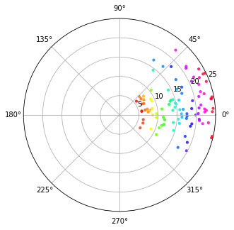
The answer was to convert the polar degrees to radians and then to a complex number. I simulated wind speed and wind direction using Gaussian noise in this Jupyter Notebook, and centred the data around 10° with a variance of 20º. Python handles the basic math required to calculate the mean wind direction seamlessly and there are also libraries available for MCUs such as Arduino to do the same thing.
Whenever you have real-world data input, it’s going to have some amount of noise. Dealing with that noise properly can make a huge difference in the behavior of your robot, rocket, or weather station. How much filtering to apply is often a matter of judgement, so starting off with a simple filter like the EWMA, plotting out the data, and adjusting the smoothing parameter by eye is the easiest way to go. When that fails, you’re ready to step up to more complicated methods.